
Steve Palosh and Chris Schuermyer, Synopsys, Mountain View, cA
Pietro Babighian and Yan Pan*, GLOBALFOUNDRIES, Malta, NY
*now with Advanced Micro Devices, Inc.
Scan diagnosis is commonly used on devices that contain logic tested by ATPG (Automated Test Pattern Generation) to enable a wide range of silicon learning applications. The process involves collecting the results of a device’s digital failures from ATE (Automated Test Equipment) patterns and providing them as input to a diagnostic fault simulation. This simulation is performed on a high-volume of failing devices using the same EDA software that generated the test patterns. The physical locations and defect types determined through simulation can then be correlated with a variety of spatial locations, parametric data, or other FAB parameters. For high-level volume analysis this methodology is proven to be very productive.
At the PFA (Physical Failure Analysis) level, engineers use the output diagnostic fault simulations to assist them in localizing the physical area where a silicon defect can be found. In many cases these simulations can have ambiguous results that look like multiple candidates or defect classifications for the exact same electrical failure. Using expert knowledge, the analyst must to consider this ‘diagnostic noise’ and still choose the location that they think has the highest likelihood of being correct. If the PFA is successful, then the defect and its classification are confirmed.
Traditional equipment-based factory flows for inline inspection and PFA are expensive. For that reason, their use is highly selective and limited in the volume of devices that can be sampled. At advanced technology nodes, the capabilities of optical and e-beam inspection are becoming more limited. At more established technology nodes, the foundry may not have the budget resources to upgrade existing tools. In both cases the variety and complexity of digital content in IC designs continues to increase.
With the application of Bayesian Machine Learning, FMA (Failure Mechanism Analysis) provides yet another diagnostic signal for holistic volume diagnostic analysis. FMA processes a population of scan diagnostic results to separate the true, yield-limiting failure mechanisms from the diagnostic noise.
If done correctly, the extracted signals serve a similar purpose as a defect pareto extracted from PFA or inline inspection. In cases where volume scan fail bit data is available, a silicon defect Pareto can now be derived quickly through software at a fraction of the cost. This means the use of expensive factory flows could be reduced or complimented by failure mechanisms identified through software on large volumes of device data.
FMA example
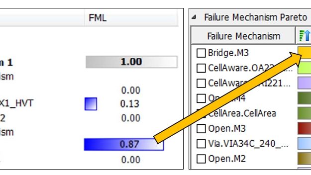
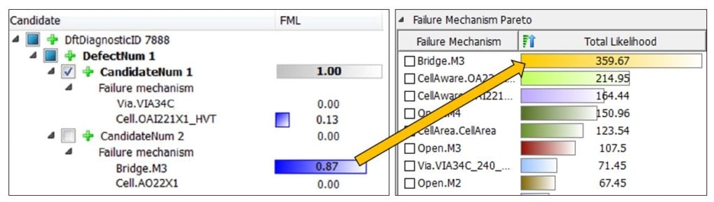
In Figure 1, diagnosis has determined that there are multiple candidates and physical details that could explain the failure. FMA gives each of these possibilities an FML (Failure Mechanism Likelihood). This FML provides the expert knowledge to the user in identifying the best candidate for PFA which in this case is Bridge.M3. Of all the mechanisms presented, the Bridge.M3 is the only one that should be counted as part of the Failure Mechanism Pareto and the Total likelihood for the Failure Mechanism Bridge.M3.

FMA advantages
FMA clusters the scan diagnosis population by failure mechanism which helps the foundry to target FA so that there is a better chance for different yield limiters to be discovered with a fewer number of PFA jobs. This provides a significant improvement in PFA cost savings and reduced turn-around time to detect a full spectrum of defects.
Conventional volume diagnosis analysis results in a multitude of signals for each type of analysis (cell outlier, metal open outlier, etc.) without a clear weight on the importance of each signal. It is difficult to share such signals with process integration or yield engineering teams, who may not be intimately familiar with the diagnosis process or the terminologies. FMA, on the other hand, provides a clear, overall failure mode Pareto that is similar to a PFA Pareto, so it is easy to digest by a wider audience.
In a foundry environment, it is common to have different process split populations to be compared for a very specific failure mode. FMA, when proven reliable with baseline wafers for detecting a specific failure mechanism, can be used to draw a quick conclusion on the process improvement wafers without having to resolve to PFA each time. This enables faster conclusions which could save cycle time associated with implementing the final process change or subsequent experiments.
FMA methodology
Bayesian machine learning is the act of reallocating credibility across possibilities as more information becomes available. The FMA model can be thought of as a probabilistic graphical model made up of four component probability distributions, which can each be described as their own probability distributions that are conditioned on some prior distribution [1].
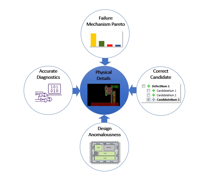
The observation data required as input to FMA comes from diagnostic reports. Scan diagnostics are generated by 4 latent factors described below.
Failure Mechanism Pareto (top in Figure 2) shows the true failure mechanism describes the physical attributes that are correlated to the defective device. For example, if the defect Pareto is estimated to only contain a single failure mechanism (because of an excursion), the failure mechanism would ideally only report the causal mechanism.
Correct Candidate (right in Figure 2) refers to the diagnostic candidate with the highest probability out of the multiple candidates that may be reported by diagnosis. Prior knowledge about the candidate’s certainty can be considered as each new candidate in the population of failing die is processed.
Design Anomalousness (bottom in Figure 2) is a measure where the larger the observed value (of the physical detail) is relative to what’s typical in the design, the higher the probability that it is responsible for the defect.

For example, imagine that a design typically has an average of 2.0 Via3’s per net. If a given diagnostic candidate net has 8 Via3’s, would be considered more anomalous with respect to Via3 than is typical. Therefore, the probability that this net is anomalous would be relatively high (compared to typical nets).
The design anomalousness parameterization employs a comprehensive characterization of the design in order to estimate what values would be considered typical.
Accurate Diagnostics (left in Figure 2) refers to the accuracy of the diagnostic fault simulations. This can involve uncertainty caused by various metadata in the diagnostics. For example, a high number of unexplained patterns by diagnosis reduces the amount of influence.
Physical Details are a fixed, observed value as reported from the Scan Diagnostics (center Figure 2). This is the only observed value in the FMA model. When the physical detail corresponds to the true physical defect the value can be thought of being drawn from a probability distribution describing the signal. When the physical detail does not correspond to the true physical defect it can be thought of as being drawn from the probability distribution of the noise.
The flow diagram of the experiments is shown in Figure 3.

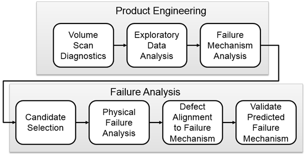
Volume Scan Diagnosis – A logic simulation is performed using the netlist, physical layout, test patterns, and the failing bits collected from ATE. Its purpose is to determine what locations in the physical design could have caused the failures. These locations are called candidates because there may be multiple locations that could cause the same test failures.
Exploratory Data Analysis – In this step the data is cleaned by removing candidates that would bias the results from the FMA methodology. Examples of candidates to be removed include those that were identified with test pattern results that were not fully explained by the simulation.
Failure Mechanism Analysis – This is where we apply the methodology that is the focus of this paper.
Candidate Selection – The Failure Mechanism Pareto provided by FMA allows selection of only the candidates that are relevant to the dominant failure mechanism of the population of all candidates being analyzed.
Physical Failure Analysis – The candidates identified in the prior step are sent to the lab where the candidates could be analyzed to see if the physical failure mechanism identified through software simulation really exists.
Defect Alignment to Failure Mechanism – This is where the failure analyst classifies the defect as one of the mechanisms that exist in the failure mechanism Pareto.
Validate Predicted Failure Mechanism – The failure mechanism predicted by FMA is compared to the PFA result.
Silicon results
Scan diagnostic data were collected on 89 diagnostic symptoms across six wafers subject to some Back-End-Of-Line (BEOL) process experiments. Consequently, manufacturing issues involving metal and/or via layers are expected but there is no clear indication as to which layer is impacted.
In Figure 4, FMA shows all wafers were likely affected by Via3 issues. Wafer 2 seems to have most of the yield loss attributed to Via3 (Via3_VH) whereas Wafer 3 and 4 are both attributing much of the yield loss to Via2 (Via2_HV and Via2).

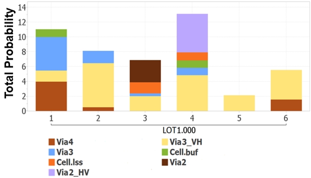
Figure 5 shows the result of PFA executed on six die from Wafer 2. FMA predictions of open defects on Via3 as the dominant signal are confirmed. A missing/undersized Via3 was found on 5 sites as shown in the table of Figure 5.

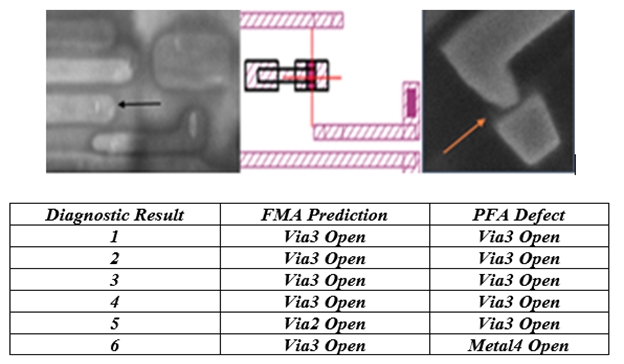
An undersized via is a good match with the FMA Via3 prediction as it is often a result of an etching problem causing the via not to properly land on the metal layer underneath, with the ultimate effect that no metal-via connection is present (Open).
While FMA is mostly successful in identifying the correct fail mechanism on the entire diagnostic population, it mispredicted two cases. In one of those cases FMA misidentified the failure mechanism as an open Via2, most likely because there is a high correlation between Via2 and Via3. In the other case, the defect was an Open M4 where FMA reported that it was an open Via3. In this, since most of the population was failing due to Via3, it was given relatively more weight compared to an open metal 4 (which only represents 1/6 of the PFA’s). It’s projected (though yet to be validated) that by bringing in historical information about the FMP, which is permitted through the form of prior knowledge in a BML model, it would be possible to correctly identify all the cases.
Conclusion
Failure Mechanism Analysis extends the value of volume scan diagnostics to deliver a failure mechanism Pareto though software which has many cost savings and productivity benefits. The role of PFA can now evolve so that it’s being used to validate the accuracy of the FMA Pareto, rather than to unilaterally estimate the defect distribution of a population.
By accurately representing diagnosis analysis results in this way, silicon results can be easily understood by many FAB teams who do not have expert knowledge of DFT, ATPG, or Silicon Diagnostics terminology.
PFA itself can be targeted more accurately to specific locations. This can reduce the number of PFA jobs required or make more PFA resources available for analysis of the defects that are not easily modeled by scan diagnostics.
References
1. C. Schuermyer, S. Palosh, P. Babighian, Y. Pan*, “Application of Bayesian Machine Learning to Create A Low-Cost Silicon Failure Mechanism Pareto,” in Advanced Semiconductor Manufacturing Conference 2019